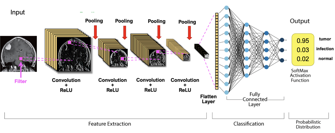
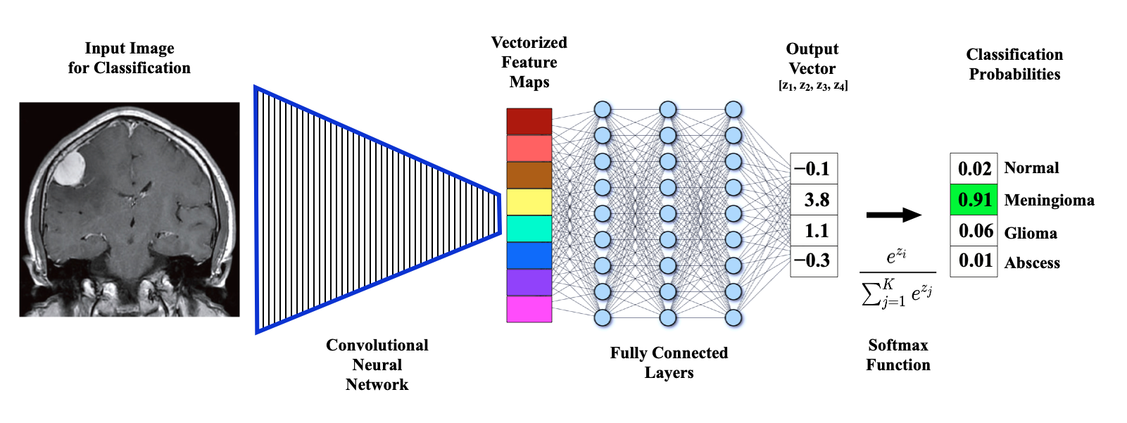
In the last several Q&A's, we have finally developed a background to understand how a convolutional neural network (CNN) is constructed. In this Q&A we will try to put the pieces all together, expanding on the diagram below representative of a series-type CNN (like VGGNet) whose input might be an MR image and output a disease prediction/classification.
|
Convolution
Convolution of the input image is the initial step in a CNN. As described in the prior Q&A, convolution involves a sliding multiplication and addition of regional data points by a small (typically 3x3 or 5x5) array of numbers called a kernel or filter. By using sets of different kernels (such as ones that emphasize edges or shapes) a set of regional feature maps is produced.
Note that during training of the network, the filters at each layer will change gradually until they are optimized for the particular purpose intended (e.g., segmentation, classification).
|
Activation
An activation function is also commonly applied during feature map generation to constrain output pixels to a certain range. As described in a prior Q&A, a common choice is the Rectified Linear Unit (ReLU) function that passes through only positive values to the feature map and sets all negative pixels to zero.
An activation function is also commonly applied during feature map generation to constrain output pixels to a certain range. As described in a prior Q&A, a common choice is the Rectified Linear Unit (ReLU) function that passes through only positive values to the feature map and sets all negative pixels to zero.
|
Pooling (Downsampling)
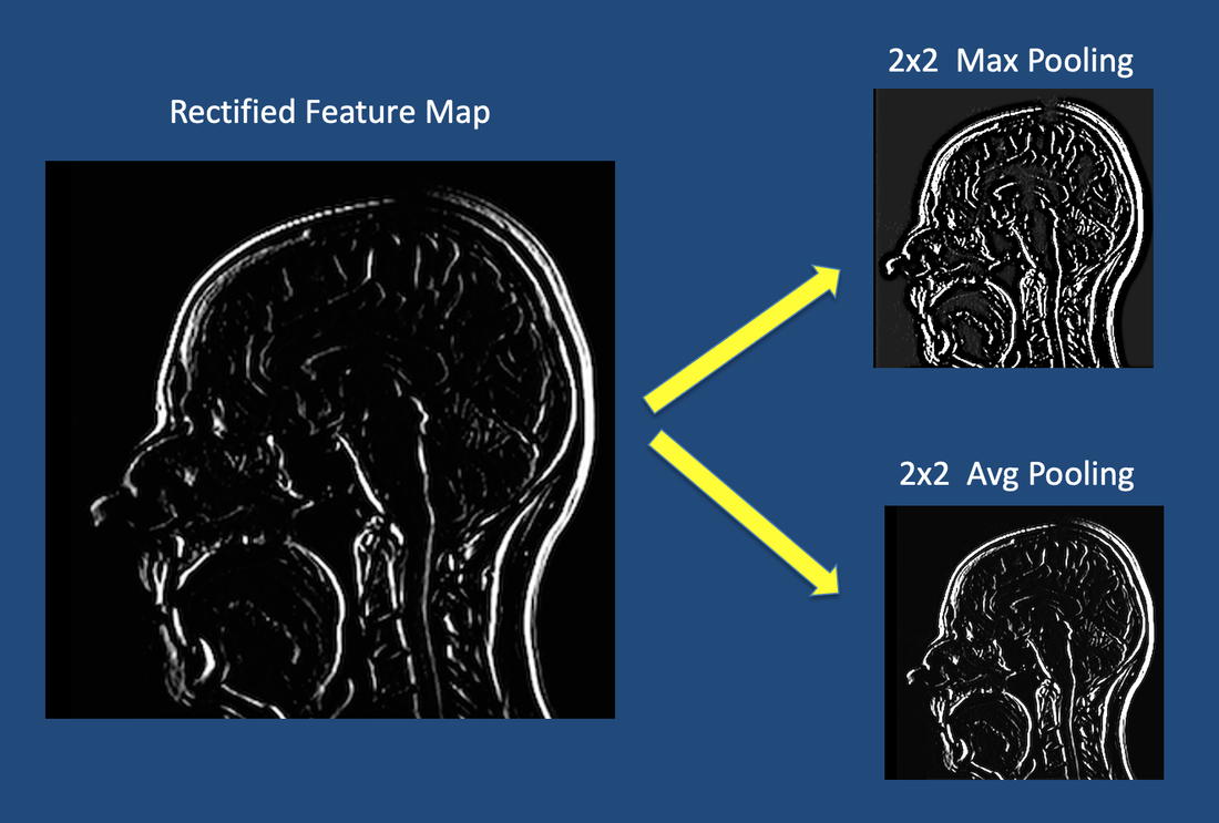
The next step, pooling, shrinks the size of each feature map by 75% or more. This allows only the most important features to be retained, thus reducing the number of learnable features of the model. With fewer parameters, pooling helps prevent overfitting of data. Pooling also reduces spatial invariance, meaning the network is able to recognize features even though they may be distorted or rotated. |
|
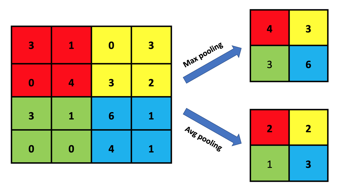
The most popular method is known as Max Pooling and uses a 2x2 filter to operate on each feature map. As shown in the illustration, the Max Pooling filter takes the largest value from each group of 4 pixels, thus shrinking the image substantially. A second common method is Average (Avg) Pooling, where the average value from each group of 4 pixels is taken. Other techniques include Min Pooling, Global Pooling, Stochastic Pooling, and 1-2 Norm Pooling.
|
Convolution, Activation, and Pooling ..... Repeat
The convolution-pooling process may be repeated several times, producing ever smaller "feature of feature" maps. Pooling is not always performed after each convolution; in some networks several convolutions are performed followed by a pooling step.
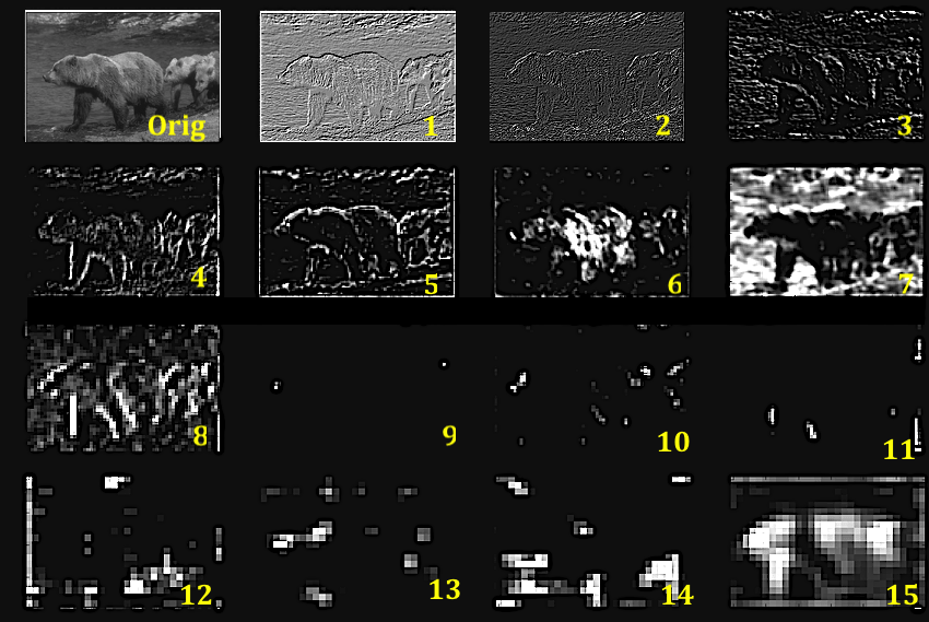
A common question that arises is what to these inner networks doing and what do deeper level feature maps look like?
Although the results depend upon the particular network under consideration and filters selected, the following statements generally apply:
- The initial feature maps reflect the presence of lines, edges, and simple regions of light and dark within localized areas of the original image spanned by the convolution kernel.
- Subsequent early layers are sensitive to curved contours and the junction of lines, recognizing loops and corners. Ultimately whole shapes like rectangles and circles may arise.
- Deeper convolutions produce maps sensitive to texture and surfaces.
- With progressive convolutions and pooling, the feature maps become progressively smaller and coarser. They are no longer localized but contain information from all parts of the original image.
- These nested "features of features" maps may become largely unrecognizable to our eyes, reflecting hidden patterns and relationships between objects detected at earlier stages.
- With training the filter weightings are modified to become optimized for the specific task required.
The image and Deep Visualization Toolbox video by Jason Yosinki below may help you get a better feeling about what the computer is "seeing" in these deeper layers.
Final Processing Steps
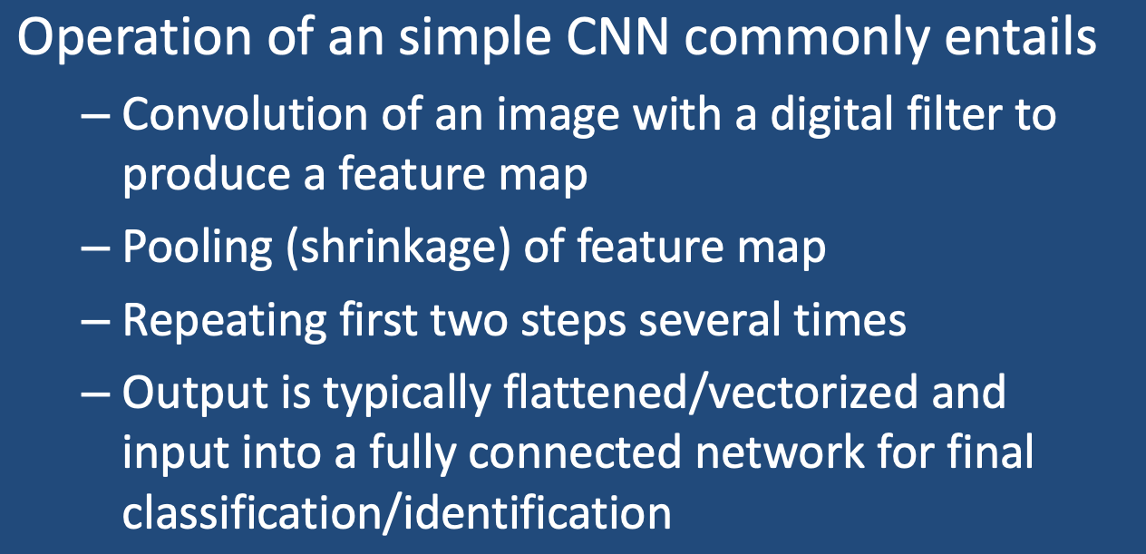
Many possibilities exist once the multiple convolution-pooling process is complete. One common final stage, known as vectorization or flattening, converts the last 2-dimensional feature maps into a single long chain of numbers (i.e., a "vector"). The vectorized feature maps then serve as inputs into a fully connected neural network whose output can be used to produce a final "decision" (such as tissue segmentation or disease classification). The fully connected layers allow the system to combine various combinations of information from the vectorized feature maps in making the system's end result. To have statistical meaning, the raw data in the output vector must be transformed into probabilities by use of the Softmax function (described in more detail in the next Q&A). Alternatively, the fully pooled data may be re-expanded back to its original dimensions, a process known as up-pooling, outlined in the a subsequent Q&A.
Advanced Discussion (show/hide)»
No supplementary material yet. Check back soon!
References
Ajit A, Acharya K, Semanta A. A review of convolutional neural networks. 2020 International Conference on Emerging Trends in Information Technology and Engineering (ic-ETITE):1-5. [DOI LINK]
Amidi A, Amidi S. VIP Cheatsheet for CS 230 - Deep Learning: Convolutional Neural Networks. Stanford University; 2019:1-5. [Downloaded from this Link 6-22-22]
Brownlee J. How to visualize filters and feature maps in convolutional neural networks. In: Deep Learning for Computer Vision. 2019:1-17.
Yosinski J, Clune J, Nguyen A, et al. Understanding neural networks through deep visualization. ArXiv 2015;1506.06579. [ArXiv Link]
Zeiler MD, Fergus R. Visualizing and understanding convolutional networks. ECCV 2014, Arxiv 13.11.2901 (Nov 28,2013) [ArXiv LINK]
Related Questions
I still don't understand how machines learn. How do they "reprogram" themselves?
What does the term convolution mean?
What is the Softmax function and why is it needed?
I still don't understand how machines learn. How do they "reprogram" themselves?
What does the term convolution mean?
What is the Softmax function and why is it needed?
