Machines "optimize themselves" by updating the weights and biases of neural network components during training through the following steps:
- Forward Pass: Training input data is fed through the neural network, passing though in a forward direction while undergoing a set of linear transformations and non-linear activations to produce one or more outputs.
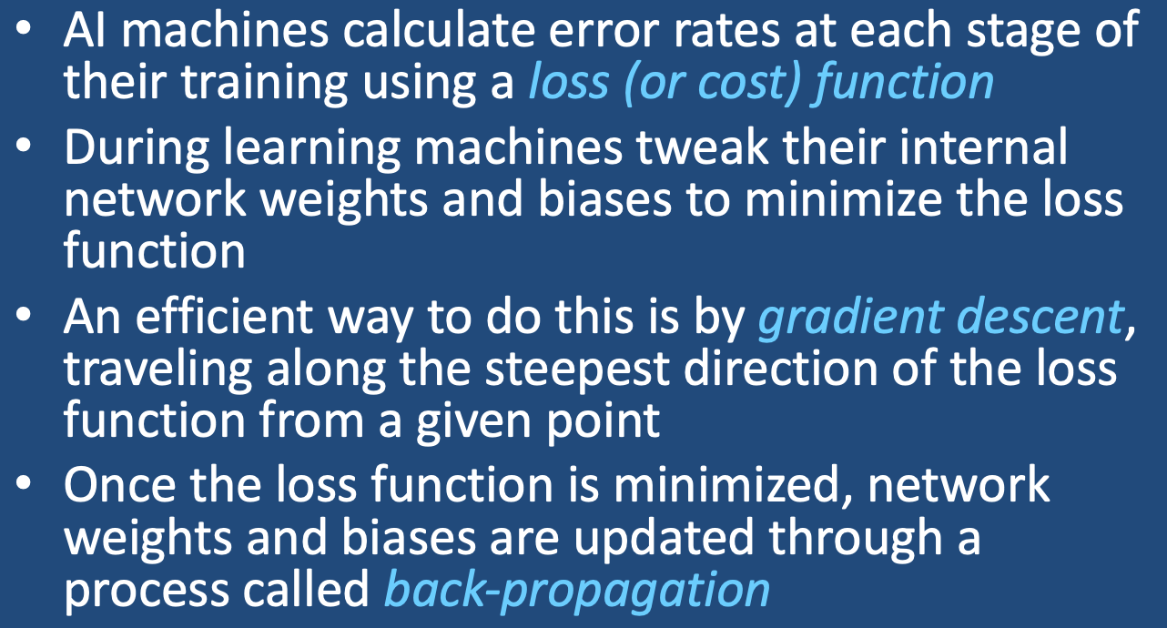
- Loss Calculation: The difference between the ideal predicted and measured value of each output is quantified by the Loss Function, introduced in a prior Q&A.
- Gradient Descent and Back-Propagation. The gradient of the loss function with respect to each weight in the network is computed using the chain rule of calculus. This gradient represents the steepest slope of the loss function at each node. The gradient is calculated by propagating the error backwards through the network, layer by layer, starting from the output layer to the input layer.
- Weight Update: The weights and biases in the network are adjusted by moving them in the opposite direction of the gradient of the loss function. This is done by subtracting a small fraction of the gradient from the current values of the weights and biases. The fraction of the gradient that is subtracted is known as the learning rate, which determines how large the weight updates are.
- Repeat: Steps 1 to 4 are repeated for multiple epochs or iterations until the network converges to a minimum value of the loss function.
Gradient Descent
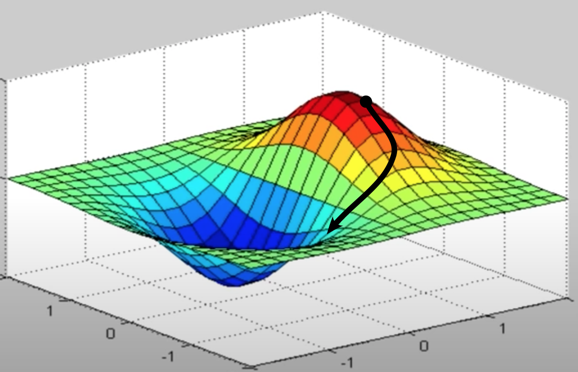
The third step in the optimization procedure, Gradient Descent, involves planning the most efficient path to minimize the loss function after each set of training data has been input into the system. This procedure has been likened to finding one's way down a mountain in the fog. At each point you search locally to see where the slope downward is steepest, then take a step in that direction and repeat. Eventually you will hopefully find your way to the bottom of the mountain and obtain the lowest global value for the loss function. Occasionally, however, you may get stuck on a flat part of the mountain (where the slope is zero in all directions) or settle into an intermediate valley (a local minimum).
To reduce computational burden several variations of the method have been developed, the most popular being stochastic gradient descent (that uses a randomly selected regional subset of the data rather than computing an exact slope/derivative at every point) and its variant Adam (that includes Adaptive moment estimation).
To reduce computational burden several variations of the method have been developed, the most popular being stochastic gradient descent (that uses a randomly selected regional subset of the data rather than computing an exact slope/derivative at every point) and its variant Adam (that includes Adaptive moment estimation).

Loss function represented in 3 dimensions. The network begins at the solid black circle with a relatively high error rate (loss). Numerical differentiation (ie, calculation of gradient/slope) of the loss function with respect to various parameter weights identifies the local path of steepest descent. At each point along the descent a new steepest gradient is calculated and the descent path modified until a minimum is reached.
A specific algorithm, back-propagation, updates network weights and biases sequentially from back to front. The details of this process are somewhat complicated, but involve use of the chain rule (from calculus) to allow gradient weights to calculated and updated one layer at a time. Once the output layer errors are calculated, the errors are propagated backward through the network. At each layer, the error is multiplied by the derivative of the activation function with respect to the weighted sum of the inputs. This gives the error at the weighted sum of the inputs to each node.
The following video serves as a useful introduction to this process.
Advanced Discussion (show/hide)»
No supplementary material yet. Check back soon!
References
Backpropagation. Wikipaedia, The Free Encyclopedia. (downloaded 3 Feb 2022)
Kingma DP, Ba JL. Adam: a method for stochastic optimization. arXIV:1412.6980v9 2017.
Le Cun Y. A theoretical framework for back-propagation. In: Touretzky D, Hinton G, Sejnowski T (eds). Proceedings of the 1988 Connectionist Models Summer School, Carnegie Mellon University, Pittsburgh PA, Morgan Kaufmann, 1988: pp 21-28.
Meeden L. Derivation of backpropagation. Course notes for CS81 - Adaptive Robotics 2010: 1-4. [Downloaded from this link 6-25-22]
Rumelhart DE, Hinton GE, Williams RJ. Learning representations by back-propagating errors. Nature (letters) 1986;323:533-5.
Sebatian. An introduction to neural network loss functions. Blog post on Programmathically 28 Sept 2021. [available at this link]
Related Questions
Is deep learning (DL) the same as machine learning (ML)?
Is deep learning (DL) the same as machine learning (ML)?
