 The "Miracle"
of k-space
In other words, each data point of the MR signal is already in "Fourier format." I call this surprising fact the "Miracle" of k-space! Why this miracle occurs is not intuitively obvious and will require some explanation.
The diagram below shows a hypothetical FID obtained from an MR slice through the upper abdomen. The FID has undergone accelerated decay due to the action of a dephasing gradient G(x) that is directed along the horizontal axis. G(x) might serve as either a frequency- or phase-encoding gradient. For simplicity we assume G(x) varies linearly with position (x), having the form G(x) = G • x, where G is expressed in mT/meter or equivalent units.
The diagram below shows a hypothetical FID obtained from an MR slice through the upper abdomen. The FID has undergone accelerated decay due to the action of a dephasing gradient G(x) that is directed along the horizontal axis. G(x) might serve as either a frequency- or phase-encoding gradient. For simplicity we assume G(x) varies linearly with position (x), having the form G(x) = G • x, where G is expressed in mT/meter or equivalent units.
While G(x) is being applied, the total magnetic field at a given location is B(x) = Bo + G(x). The corresponding resonance frequency at location x is therefore
f(x) = γB(x) = γBo + γG(x) = fo + γGx.
where γ is the gyromagnetic ratio and fo is the Larmor frequency of the main magnetic field (Bo). Under action of the gradient, the resonant frequencies increase from left-to-right across the image as long as the gradient is being applied. Once the gradient is turned off, the resonant frequencies all revert to fo.
While the gradient is applied, protons in the higher parts of the field will precess more rapidly and gain phase compared to those in lower parts of the field. This phase shift persists even after the gradient has been turned off. Because phase = frequency x time, the phase gain is directly proportional to the length of time (t) the gradient is applied. As a function of position (x), the phase gain is given by
ϕ(x,t) = (γGx) • t = (γGt) • x = kx(t) • x
where kx(t) = γGt. This is the same "kx" of k-space fame, expressing phase cycles per unit distance along the x-direction.
Another way to think of k(t) is as the gyromagnetic ratio (γ) times the area under the gradient (G) curve at time (t). Even though we have assumed a linear, rectangular gradient waveform varying along the x-axis in our simplified example above, the same definition holds for any arbitrary gradient shape and direction (r). Specifically,
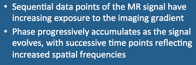
When t = tearly, kx is small and the spread of phases across the image is very small. When t = tlate, kx is large and many phase cycles encompass the image. The resultant MR signal at each point in time (t) thus reflects increasing spatial frequencies and the summed phase angles from all locations in the image. Hence each successive point along the MR signal reflects progressively higher spatial frequencies whose values can be used to "miraculously" fill k-space cells directly.
|
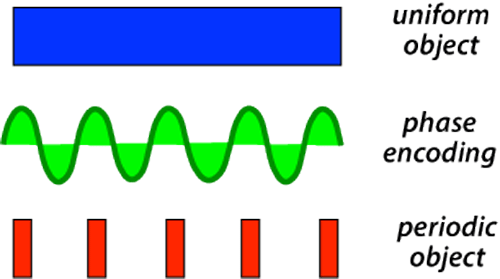
If the above discussion was too mathematical, perhaps the example left will provide some additional insight. Here two objects, one of uniform density (blue) and the other of periodic density (red, like a fence), have been subjected to the same gradient field. We assume this gradient has induced a set of phase shifts (green) across both objects, whose spatial frequency happens to match that of the red object.
|
Because the uniform (blue) object extends over multiple phase cycles, no signal would be observed as magnetization vectors would all cancel. In other words, for each pixel in the uniform object with phase shift φ, it would be easy to find another pixel with phase shift −φ. Conversely, the red object would generate a strong signal at this phase encoding, as the spatial frequency inherent in the object would exactly match that produced by the gradient.
Advanced Discussion (show/hide)»
No supplementary material yet. Check back soon!
References
Mezrich R. A perspective on k-space. Radiology 1995; 195: 297-315 [review].
Wald L. MR image encoding. (From MIT OpenCourseWare http://ocw.mit.edu)
Mezrich R. A perspective on k-space. Radiology 1995; 195: 297-315 [review].
Wald L. MR image encoding. (From MIT OpenCourseWare http://ocw.mit.edu)
Related Questions
Where do you get the data to fill k-space? How does this relate to MR signals and echoes?
Where do you get the data to fill k-space? How does this relate to MR signals and echoes?


